
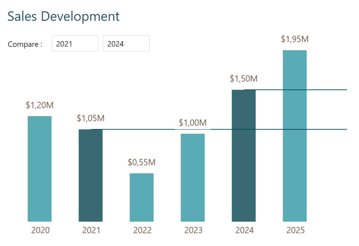
When analyzing data over time, the most common need is simple: show the difference between a starting period and an ending period. But what happens when the user wants to choose those periods themselves?
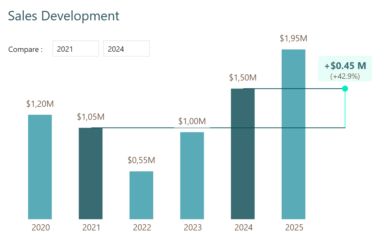
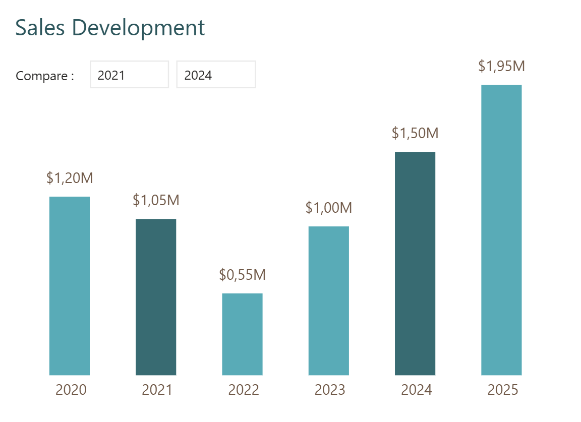
That is where it gets interesting and tricky. This chart lets the user pick a starting year and an ending year, and visualizes the difference cleanly on the right-hand side. It is a great example from a UX standpoint, and it is packed with technical tricks.
Fair warning: from a technical point of view, this is not an easy one. But once it works, it is really satisfying.
Fair warning: from a technical point of view, this is not an easy one. But once it works, it is really satisfying.
What we are building
The chart has several components working together:
- A slicer where the user can choose a starting year and an ending year
- Conditional formatting that highlights the selected start and end years in different colours
- Two horizontal lines that extend from the selected years to the right-hand side of the chart
- A vertical connecting line between those two horizontal lines
- A data label showing the absolute difference and the percentage difference
- Extra space on the right-hand side of the chart where all of this is visualised
Each of these requires its own trick. Here is how to build them one by one.
Step 1: Create a disconnected slicer table
The first question is: why doesn't the slicer filter the column chart below it? Normally a slicer filters everything. But in this case, 2020 and 2025 still show up in the chart even when they are not selected in the slicer. That is intentional and it is achieved by using a disconnected table.
In the data model, create a table called dimDate slicer. This table is not connected to any other tables. It simply returns a list of all the years in your dim date table, using a formula like this:
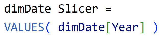
Once you have this table, build your slicer from it:
- Insert a slicer and use the Year field from dimDate slicer
- Remove the slider style - a simple list works better here
- Turn off the header
- Reduce the text size and resize the slicer to fit
- Turn off the background
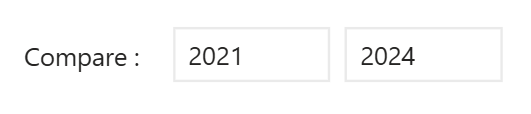
- Add a text box next to it with the word "Compare" to label it clearly
Now go to Format, Edit Interactions, and make sure the slicer is set to filter the column chart. It will not visually change what years show, but the visual still needs to know which years are selected. That filter interaction is what makes the rest of the measures work.
Step 2: Create space on the right-hand side
The connecting lines and data label need space to live on the right hand side of the chart. There is no formatting option that creates this space directly. Hence, the trick is to add placeholder year.
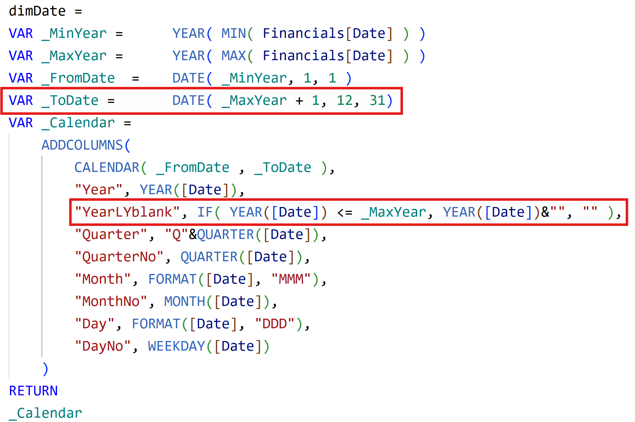
In your calendar table, make two small changes:
- Extend the end date of the table by one year. First calculate the max year in your dataset - in this example that is 2025, then add one year. So if your data goes to 2025, your date table goes to 2026.
- Add an extra column called Year Last Year Blank. For dates in the year 2026, this column returns blank. For all other years, it returns the respective years.
Make sure the YearLYblank column is a text column - you cannot mix data types in one field, so add a small text conversion to the year values to keep everything consistent.
Back in the chart,
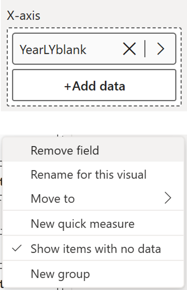
- add YearLYblank to the x-axis.
- Right-click on the field and select Show Items With No Data.
- The blank space will appear on the right-hand side.
- Set the sort by column for Year Last Year Blank to Year, sorted in ascending order.
Step 3: Apply conditional formatting to highlight selected years
Create a measure called CF that returns a 1 or a 0 depending on whether the year on the horizontal axis matches the minimum or maximum year selected in the slicer:
Create a measure called CF that returns a 1 or a 0 depending on whether the year on the horizontal axis matches the minimum or maximum year selected in the slicer:
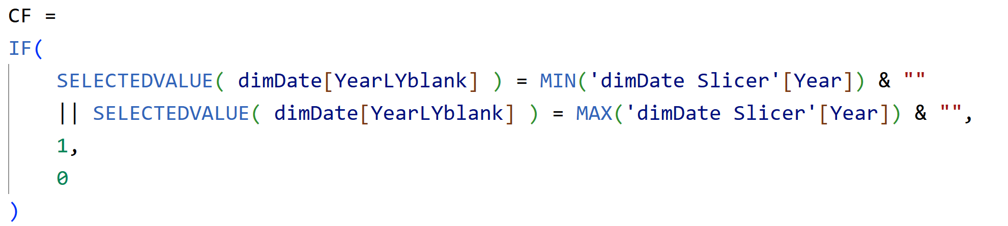
Watch the data types here - the year values in the measure need to match the text format used in the Year Last Year Blank column.
Apply this to the column chart:
- Select the chart and go to Formatting
- Under Columns, open the Color conditional formatting
- Choose Rules
- Select the CF measure
- Set the rule: if CF is equal to 1, apply a highlight colour
You should now see the selected start and end years highlighted in the chart. Consider adding a visual level filter on the Year field if you do not want users to be able to select the placeholder year 2026.
Step 4: Draw two horizontal lines
To draw the horizontal lines from the selected years to the right-hand side, you need two measures: one for the minimum year and one for the maximum year.
To draw the horizontal lines from the selected years to the right-hand side, you need two measures: one for the minimum year and one for the maximum year.
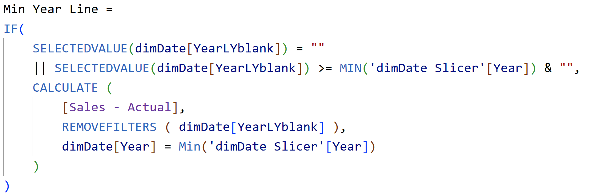
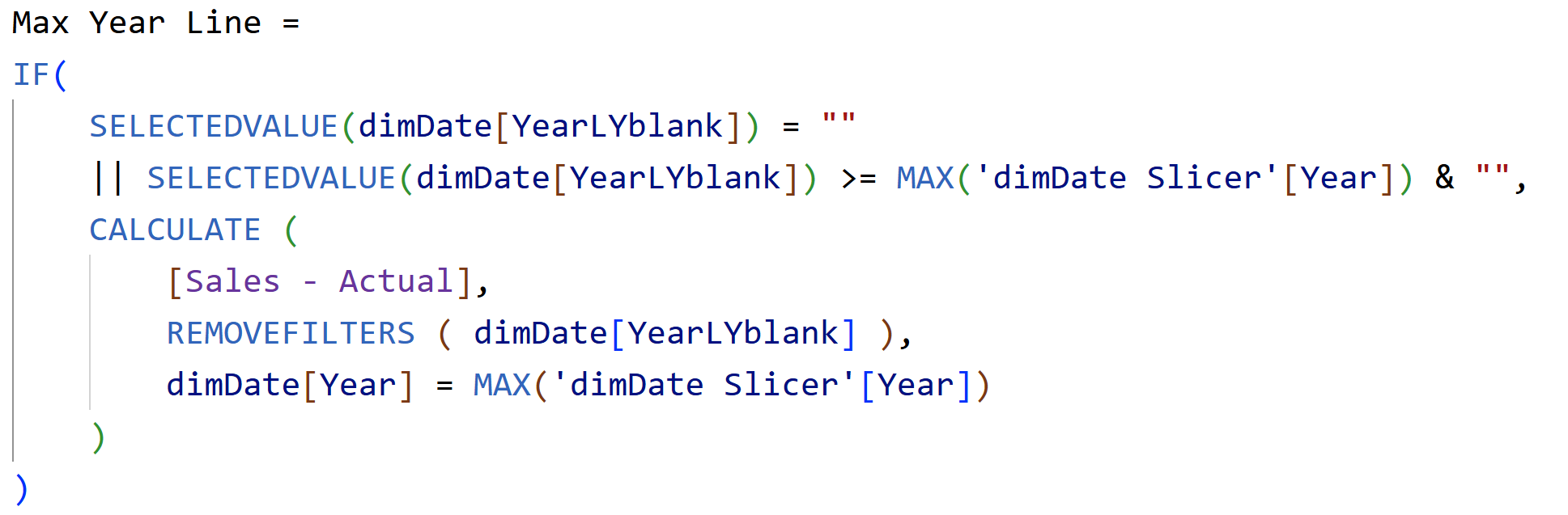
The min year line measure works like this:
- Use a CALCULATE function to remove the filter coming from the Year Last Year Blank field on the x-axis
- Replace it with a filter where Year equals the minimum year selected in the slicer
- This gives you the sales actual value for that minimum year
- Then wrap it in an IF function: only return that value where Year Last Year Blank is equal to or greater than the minimum year selected in the slicer - so the line draws from that year all the way to the right
The max year line measure does exactly the same thing but uses the maximum year selected in the slicer.
To add these to the chart:
- Change the chart type from a column chart to a line and clustered column chart
- Add min year line and max year line to the line y-axis
- Turn off the legend
- Turn off data labels for both line series
- Make the lines thinner and set them to a neutral colour such as light gray
Test it - change the starting year in the slicer and the line should jump to the correct year. Change the ending year and the same happens.
Step 5: Draw the vertical connecting line using error bars
You cannot draw vertical lines in a line chart directly. The workaround is to use error bars.
You cannot draw vertical lines in a line chart directly. The workaround is to use error bars.
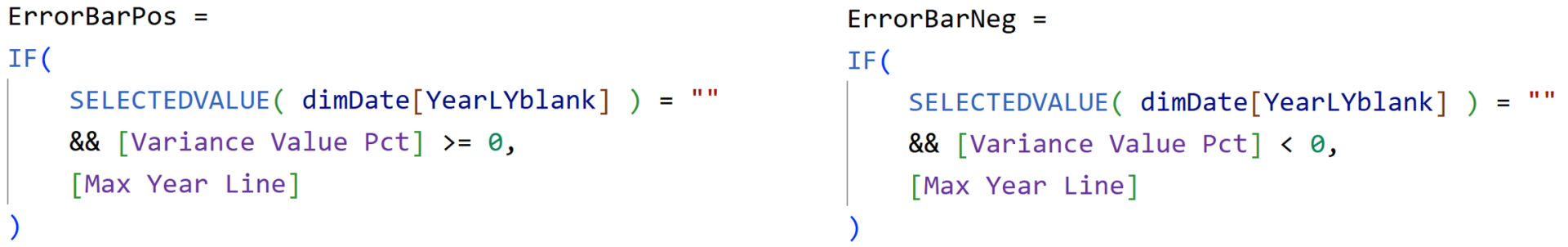
Create two measures: Error Bars Positive and Error Bars Negative. Both measures check whether we are in the placeholder year 2026 - if so, they return the max year line value. The difference between them is the condition that checks the sign of the variance, which allows the connecting line to appear in a different colour depending on whether the difference is positive or negative.
Add Error Bars Positive to the line y-axis first. Then:
- Go to Lines and change the colour to your preferred colour for positive variance
- Go to Markers, turn them on, and adjust the size as you like
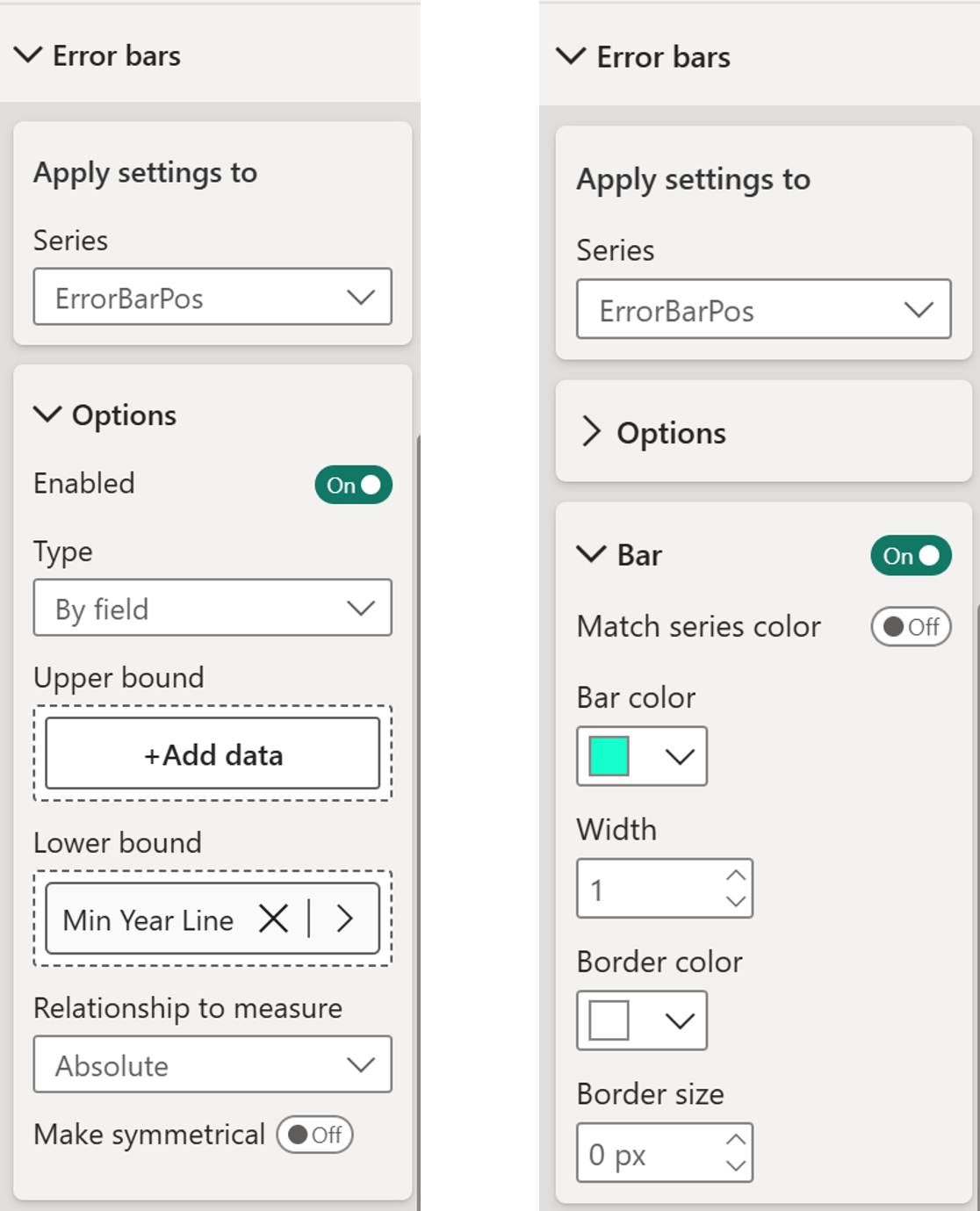
- Go to Formatting and open Error Bars for the Error Bars Positive series
- Enable error bars and set the lower bound to min year line
- Go to Bars, turn it on, and set the bar colour - green works well for positive variance
- Set the border size to zero to make the bar thinner
Now add Error Bars Negative to the line y-axis and repeat exactly the same steps - change the line colour, set up the error bars with min year line as the lower bound, and set the bar colour for negative variance.
You should now see the vertical connecting line between the two horizontal lines for both positive and negative variance scenarios.
Step 6: Add the data label
With the error bars in place, add data labels to both series.
With the error bars in place, add data labels to both series.
For Error Bars Positive:
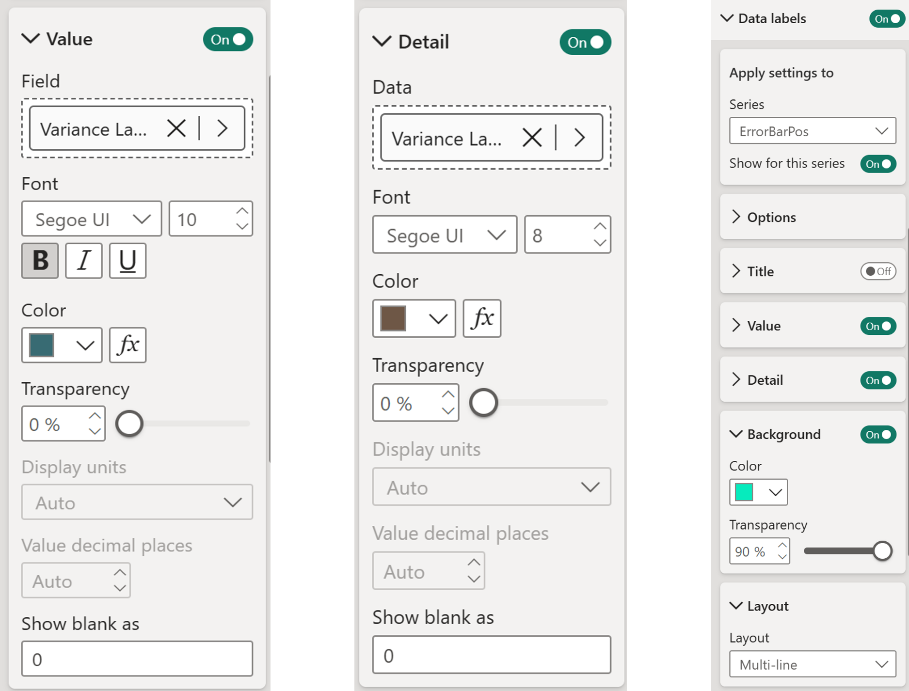
- Go to Data Labels and select the Error Bars Positive series
- Set the layout to Multi-line, you need to select this explicitly, it does not default to it
- Under Value, set up two parts:
Title - use your label title measure for the absolute difference
Detail - use your percentage difference measure - Go to Background, apply the green colour with a little transparency
- Make the percentage text slightly smaller than the absolute value above it
- Make the absolute value bold or larger if you prefer
For Error Bars Negative, apply exactly the same data label settings - same layout, same title and detail setup, same background treatment. Note that when the variance is negative, the secondary y-axis may appear. Turn it on and off again to clear it.
And there you go!
This is not a simple build - a disconnected slicer table, a placeholder year in the date table, a line and stacked column chart, error bars used as vertical connectors, and multi-line data labels all working together. But that is also what makes it satisfying when it comes together. The end result is a chart that gives users genuine control over which periods they are comparing, with the difference visualised cleanly and clearly right where they are looking.
Hope you like it!
Hope you like it!
Give it a try and see how it works for you! I’d love to hear what you think or see how you use this trick in your own reports.
How to Power BI
Watch it here

COMPANY
Write your awesome label here.
Embedding Power BI in Power Point
Intro Session